Key Takeaway

I want to share some of my findings from reading “Causal Inference: The Mixtape”. The biggest of which is that if you include the wrong variables, the entire coefficient direction could be flipped (going from negative to positive). This means we need to take extra care when trying to make decisions based off of data, especially if we’re not sure if we’ve included colliders.

Background

For this blog post, I’m going to focus on some of my findings from reading Chapter 3 of “Causal Inference: The Mixtape”, which can be found here: https://mixtape.scunning.com/03-directed_acyclical_graphs

First, let’s get some simple notations out of the way.

In the following DAG, it’s saying that D causes Y, and X causes D and Y. 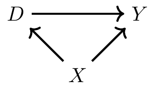In this diagram, X is a confounder. If we do not include it in a model when attempting to understand the effects of D on Y, we’ll get an inaccurate result, as we’ll sometimes pick up on spurious correlations due to the effect of X on both D and Y.

However, sometimes we cannot observe all the confounding variables, and that is represented by a dashed line. 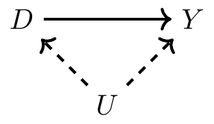In this case, because we cannot observe U, we cannot control it. That means that we cannot close the backdoor path and satisfy the backdoor criterion (which means that we are unable to accurately read the effects of D on Y because of omitted variable bias).

Even more insidious are colliders, which is where two variables both affect a third variable, as shown in this DAG: 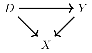Colliders, when left alone, always close a backdoor path. However, when you include them in a model, it actually opens up a backdoor path and could completely invert the coefficients.

Test on Synthetic Data, Especially the Effect of Colliders

The data we’ll look at is a synthetic dataset of female discrimination on wages. From the original text. For instance, critics once claimed that Google systematically underpaid its female employees. But Google responded that its data showed that when you take “location, tenure, job role, level and performance” into consideration, women’s pay is basically identical to that of men. In other words, controlling for characteristics of the job, women received the same pay. But what if one of the ways gender discrimination creates gender disparities in earnings is through occupational sorting? If discrimination happens via the occupational match, then naïve contrasts of wages by gender controlling for occupation characteristics will likely understate the presence of discrimination in the marketplace.

The below DAG is from the book. I will briefly summarize the DAG and go over the data generating functions, and talk about what it means when we try to extract causal impacts from models.

Let me start by going over the Causal DAG we’re using, and explaining some of the concepts here: 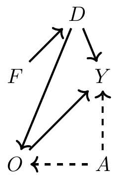First, some explanations on the variables:

• F stands for Female, and it directly influences discrimination (i.e. Discrimination is 1 whenever Female is 1)
• D stands for discrimination- in this example, it is a binary variable
• O stands for Occupation- in this example, it will be a numeric variable (you can think of it as, the higher the number, the better the occupation)
• A stands for Ability. Notice the dotted lines- it is saying that we cannot directly observe Ability.
• Y is the dependent variable, which in this case is Wages So to understand this graph, we’re saying that being female causes discrimination. Discrimination also affects wages directly, but it also affects wages through Occupation. Also, note Ability very carefully. It is an unobserved variable that affects wages. However, Occupation is acting as a “collider” for both Discrimination and Ability, meaning that if we include it but don’t include Ability, we actually introduce bias into the coefficients.

For me, it was a bit hard to understand without some examples, so let’s dive into what we see.

Code Examples

What Do We See from the Book?

Below is the code to generate the data. Note that female and ability are completely independent of each other, as they are both random variables with no relation to each other. Discrimination is a carbon copy of female. Occupation depends on Ability and also Discrimination- notice that being Female technically doesn’t affect Occupation except through Discrimination. And lastly, Wage is a function of Occupation, Discrimination, and Ability. The coefficients in each function are the true impact of each variable on the respective dependent variable, and ideally we will be able to see that through our model:

import numpy as np 
import pandas as pd 
import statsmodels.api as sm 
import statsmodels.formula.api as smf 
from itertools import combinations 
import plotnine as p
from stargazer.stargazer import Stargazer

# read data
import ssl
ssl._create_default_https_context = ssl._create_unverified_context
def read_data(file): 
    return pd.read_stata("https://github.com/scunning1975/mixtape/raw/master/" + file)



tb = pd.DataFrame({
    'female': np.random.binomial(1, .5, size=10000),
    'ability': np.random.normal(size=10000)})
tb['discrimination'] = tb.female.copy()
tb['occupation'] = 1 + 2*tb['ability'] + 0*tb['female'] - 2*tb['discrimination'] + np.random.normal(size=10000)
tb['wage'] = 1 - 1*tb['discrimination'] + 1*tb['occupation'] + 2*tb['ability'] + np.random.normal(size=10000) 



lm_1 = sm.OLS.from_formula('wage ~ female', data=tb).fit()
lm_2 = sm.OLS.from_formula('wage ~ female + occupation', data=tb).fit()
lm_3 = sm.OLS.from_formula('wage ~ female + occupation + ability', data=tb).fit()


st = Stargazer((lm_1,lm_2,lm_3))
st.custom_columns(["Biased Unconditional", "Biased", "Unbiased Conditional"], [1, 1, 1])
st

Results:

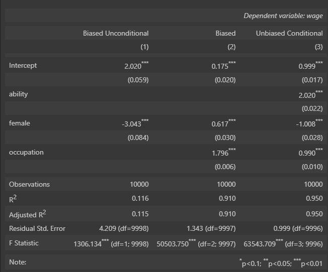
Here’s how to read this. On the top, we see each of the different runs. On the left hand side, we see a list of the variables, and then a coefficient for that variable if it was included in that run. Then on the bottom, we see the R^2 and other model performance metrics for each of the runs.

First, we see the run with only female as “Biased Unconditional”. This one shows a dramatic negative coefficient for female; however, the effect is much greater than we expect given how we made our data. Secondly, we see what happens once we include Occupation. The sign of Female FLIPs entirely! Accounting for Occupation without accounting for Ability somehow completely inverts the effects of discrimination.

Once we include Ability, we see the true coefficients appear that are very close to how we made our numbers. But, remember that Ability technically is an unobserved variable, meaning that in the real world, we do not actually know what it is.

What does this mean for us as DS? It means that, unless we fully understand what our Causal DAG would look like, we have to take any causal effects that we get from models with a grain of salt. I’m not saying that we shouldn’t try- especially for Sales, we often have no other way to understand causal effects than through running models on historical data. However, it would be wise to at least think through a Causal DAG first, and then iterate with the stakeholders if/when we find unintuitive results.

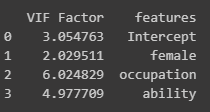
If We Look at the Correlation and VIF, We Would Actually See Occupation and Ability Are Highly Correlated and We Might’ve just Dropped One Variable

This shows that we can’t really understand what variables should be and shouldn’t be in the model based just on the correlations and VIF.

## calculate VIF of regressing on wage
from statsmodels.stats.outliers_influence import variance_inflation_factor
from patsy import dmatrices
formula = 'wage ~ female + occupation + ability'

# Get the design matrices
y, X = dmatrices(formula, tb, return_type='dataframe')

# Calculate VIF for each explanatory variable
vif = pd.DataFrame()
vif['VIF Factor'] = [variance_inflation_factor(X.values, i) for i in range(X.shape[1])]
vif['features'] = X.columns

print(vif)

Also, Regularization Should also Be Used Sparingly when Determining Causal Effects. In This Example, it Completely Removed the Coefficient from Female, Indicating that Female Did not Have Any Relationship with Wage

## Create a L1 regularized regression using the Lasso sklearn package
from sklearn.linear_model import Lasso
from sklearn.pipeline import make_pipeline

pipe = make_pipeline(Lasso(alpha=0.1))
pipe.fit(X, y)
## Get the coefficients with the column names
coefs = pd.DataFrame(pipe.named_steps['lasso'].coef_, index=X.columns, columns=['coefficients'])
print(coefs)

XGBoost and SHAP Don’t Really Fare Any Better

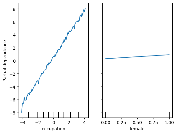
If we just regress on occupation,female in XGBoost, we see the same trends, where being female is positively associated with wage, even though we know that’s not true.

X = tb[['occupation','ability','female']]
y = tb['wage']
from xgboost import XGBRegressor
xbg = XGBRegressor()
xbg.fit(X, y)

## Create a SHAP explainer
import shap
explainer = shap.TreeExplainer(xbg)
shap_values = explainer.shap_values(X[['occupation','female']])
## Plot the SHAP values
shap.summary_plot(shap_values, X[['occupation','female']])

## Create pdp plot
from sklearn.inspection import PartialDependenceDisplay
import matplotlib.pyplot as plt
tree_disp = PartialDependenceDisplay.from_estimator(xbg, X[['occupation','female']], ['occupation', 'female'], kind='average')
plt.plot()

Other Tests

What if We Have a Random Variable that Affects Wage, but Doesn’t Affect Any other Variable?

For this test, I made up a variable called “economy” that doesn’t affect occupation or female/discrimination at all, but only affects Wage.

tb = pd.DataFrame({
    'female': np.random.binomial(1, .5, size=10000),
    'ability': np.random.normal(size=10000),
    'economy': np.random.normal(size=10000)})  # Add 'economy' variable
tb['discrimination'] = tb.female.copy()
tb['occupation'] = 1 + 2*tb['ability'] + 0*tb['female'] - 2*tb['discrimination'] + np.random.normal(size=10000)
tb['wage'] = 1 - 1*tb['discrimination'] + 1*tb['occupation'] + 2*tb['ability'] + 1*tb['economy'] + np.random.normal(size=10000)  # Add 'economy' to 'wage' equation



lm_1 = sm.OLS.from_formula('wage ~ female', data=tb).fit()
lm_2 = sm.OLS.from_formula('wage ~ female + occupation', data=tb).fit()
lm_3 = sm.OLS.from_formula('wage ~ female + occupation + ability', data=tb).fit()
lm_4 = sm.OLS.from_formula('wage ~ female + occupation + ability + economy', data=tb).fit()


st = Stargazer((lm_1,lm_2,lm_3,lm_4))
st.custom_columns(["Biased Unconditional", "Biased", "Unbiased Conditional", "Test"], [1, 1, 1,1])
st

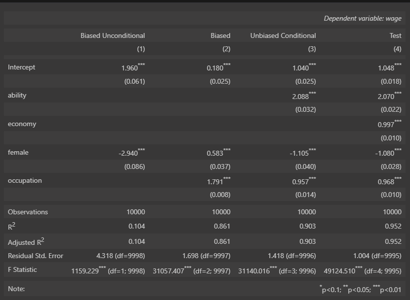
From the results, we can see that the difference between having female + occupation + ability and female + occupation + ability + economy is only based on the R^2 observed. Most of the other coefficients are very similar to what the true values are. This suggests that although predictive accuracy might decrease, if the missing variables don’t affect other variables that we are curious about, we can still trust our coefficients.

What if Discrimination Didn’t Affect Wage Directly, just through Occupation?

For this test, I removed discrimination’s direct effect on wage (i.e. I removed the D->Y edge from the DAG).

tb = pd.DataFrame({
    'female': np.random.binomial(1, .5, size=10000),
    'ability': np.random.normal(size=10000),
    'economy': np.random.normal(size=10000)})  # Add 'economy' variable
tb['discrimination'] = tb.female.copy()
tb['occupation'] = 1 + 2*tb['ability'] + 0*tb['female'] - 2*tb['discrimination'] + np.random.normal(size=10000)
tb['wage'] = 1  + 1*tb['occupation'] + 2*tb['ability'] + 1*tb['economy'] + np.random.normal(size=10000)  # Add 'economy' to 'wage' equation



lm_1 = sm.OLS.from_formula('wage ~ female', data=tb).fit()
lm_2 = sm.OLS.from_formula('wage ~ female + occupation', data=tb).fit()
lm_3 = sm.OLS.from_formula('wage ~ female + occupation + ability', data=tb).fit()
lm_4 = sm.OLS.from_formula('wage ~ female + occupation + ability + economy', data=tb).fit()


st = Stargazer((lm_1,lm_2,lm_3,lm_4))
st.custom_columns(["Biased Unconditional", "Biased", "Unbiased Conditional", "Test"], [1, 1, 1,1])
st

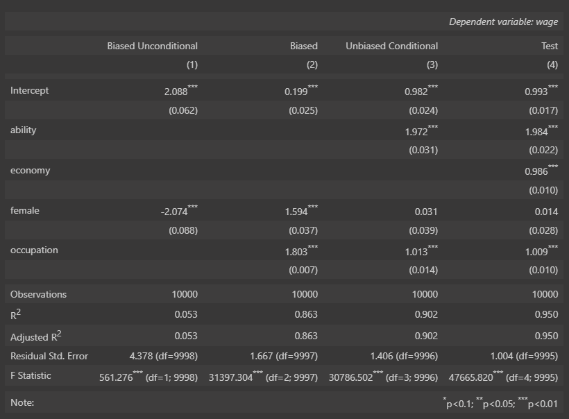
What is really interesting here is that, once we account for ability and economy, Female shows no relationship at all to predicting wage (a coefficient of 0). Even though we know that Discrimination affects Female’s ability to get better occupations, once we account for Occupation, there is no affect on Wage anymore. So we might conclude that there is no discrimination against females, when in fact it just occurs earlier up the chain.

What if Discrimination Didn’t Affect Occupation, just Wage?

Kinda the opposite of the above. Suppose that discrimination didn’t impact occupation at all (aka females and males are just as likely to get the same jobs).

tb = pd.DataFrame({
    'female': np.random.binomial(1, .5, size=10000),
    'ability': np.random.normal(size=10000),
    'economy': np.random.normal(size=10000)})  # Add 'economy' variable
tb['discrimination'] = tb.female.copy()
tb['occupation'] = 1 + 2*tb['ability'] + 0*tb['female'] + np.random.normal(size=10000)
tb['wage'] = 1 - 1*tb['discrimination'] + 1*tb['occupation'] + 2*tb['ability'] + 1*tb['economy'] + np.random.normal(size=10000)  # Add 'economy' to 'wage' equation



lm_1 = sm.OLS.from_formula('wage ~ female', data=tb).fit()
lm_2 = sm.OLS.from_formula('wage ~ female + occupation', data=tb).fit()
lm_3 = sm.OLS.from_formula('wage ~ female + occupation + ability', data=tb).fit()
lm_4 = sm.OLS.from_formula('wage ~ female + occupation + ability + economy', data=tb).fit()


st = Stargazer((lm_1,lm_2,lm_3,lm_4))
st.custom_columns(["Biased Unconditional", "Biased", "Unbiased Conditional", "Test"], [1, 1, 1,1])
st

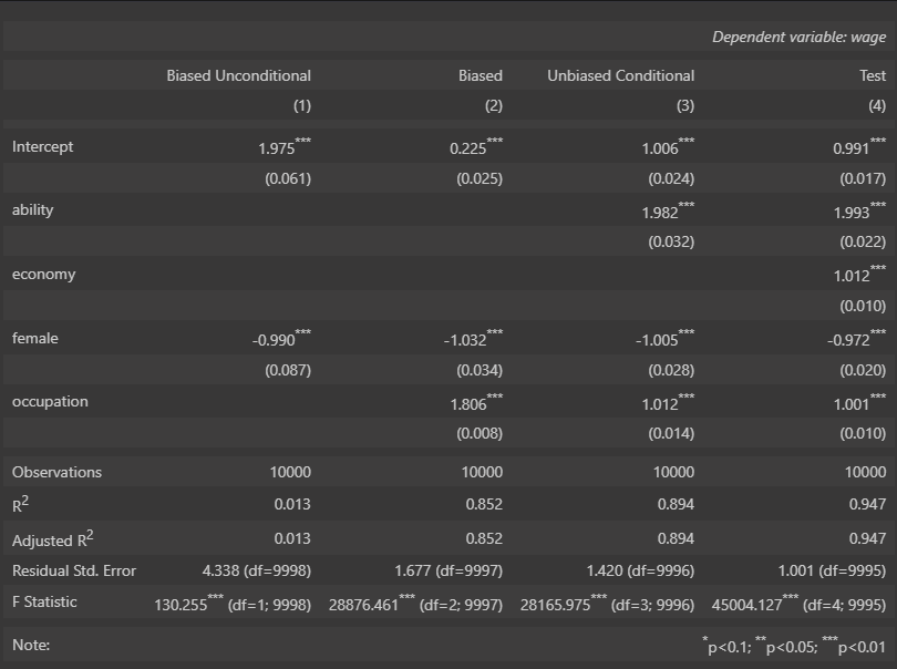
What’s interesting here is that even if we leave out occupation and ability, we still see the correct coefficient for Female.